Audio visual Speech Modeling for Continuous Speech Recognition
Introduction
Learning disabilities, vision problems, physical disabilities are the barriers to achieve the goal in this digital world. Thus, to improve the learning system, Automatic Speech Recognition (ASR) is very helpful for students with disabilities. The application area of a speech recognition system is widespread in real-time. Disabled people can use the ASR system for computing and searching on a hands-free device. They can easily access the computer, improve writing through speech to text mechanism, and increase reading-writing abilities. In voice dialing, medical documentation, home appliances, automatic speech recognition is used widely (Debnath & Roy, 2018; Revathi et al., 2019). However, the acoustic speech signal can be influenced by the transmission channel, use of the different microphones, different filter characteristics, limitation of frequency bandwidth, etc. Although there are many approaches to overcome certain situations and provide robust speech recognition, all need to know is pattern and level of noise in advance. Thus, another approach that can be used to recognize speech in the presence of acoustic noise is lipreading. The visual signal can provide speech information when an acoustic signal is corrupted by noise. Incorporating visual information into audio signal increases the possibility of a more reliable recognition system. In automatic speech recognition, visual speech helps to improve the recognition rate when background noise is more. The AV-ASR system can be used to developed desktop applications that involve web browsing tasks, air traffic control rooms, hands-free computing, where a user can interact with machines without the use of their hands. Hands-free computing is very useful for disabled people. However, primarily ASR has been used to build such applications in a noisy environment, AV-ASR can provide better performance in those application areas. Thus, providing better learning platform for physically challenged people is the prime focus of this research.
Production and perception of human speech are bi-model which include the analysis of the uttered acoustic signal and visual cues of the speaker (Dupont & Luettin, 2000). The human can use visual cues, which is the process of knowing speech by watching the movement of the speaker's lips. Most of the ASR systems apply only audio signal and ignore visual speech clues (Dupont & Luettin, 2000). It has been successfully proved that visual information of speech improves the robustness of noise in ASR. Therefore, it is very promising to cover the use of visual speech in the man-machine interaction system. However, the extraction of the visual information is challenging because the visual articulations are less informative and different from speaker to speaker (Borde et al., 2014). Moreover, visual information can also be affected by different lighting conditions. Therefore, the detection of informative visual features is still challenging. The development of AV-ASR systems must follow a better understanding of human speech perception. The following issues might be addressed while developing an AV-ASR.
- 1.
What are the benefits of visual information in speech perception?
- 2.
Which visual features are the most significant for lip reading?
- 3.
Which features provide the discriminative information to recognize different speech?
- 4.
Whether the extracted visual units are equivalent to phones?
- 5.
Whether the visual features are robust to rotation and scale?
- 6.
Whether the captured visual features are robust to different lighting conditions?
- 7.
What are the methods of integrating two information sources?
The solution to these issues could help to develop proposed AV-ASR model which improves the performance of the system. In this proposed system, visual speech recognition is added to improve the education system for disabled people. Physically challenged people can communicate with the system through audio-visual speech (Erber, 1975). The proposed system processes both the audio and visual speech signals and recognize the speech. If the audio signal deteriorates then the system will consider the visual modality. For visual speech recognition, the research proposes appearance and co-occurrence statistical measures for visual features. Accessing data is also very important for audio-visual research. A new table based protocol for data accessing in cloud computing has been proposed in many research (Namasudra & Roy, 2017). The motion of lip movement, i.e., dynamic feature provides the significant information of visual speech (Sui et al., 2017). Dynamic feature extraction and co-relation analysis of features are other important factors for differentiating speech. Co-relation analysis of visual features provides discriminatory information of the different speech, which has not been addressed by the researchers. Gao et al. (2021) proposed a novel approach on residential building load forecasting. Zhao et al. (2009) calculated LBP-TOP features for visual speech recognition. But the co-occurrences values of frames have not been considered which is very important to distinguish different frames. The appearance-based features extracted from Local Binary Pattern (LBP) and LBP-TOP are sensitive to illumination and pose. Thus, these features are not robust in environment variations. Jafarbigloo and Danyali (2021) proposed a Convolutional Neural Network (CNN) technique in which Long Short-Term Memory (LSTM) has been used for image classification. Rauf et al. (2021) introduced an optimized LSTM technique that has been used to enhance bat algorithm for COVID-19. The visual features should be illumination invariant because input data is video and variation in lighting conditions affects the different frames. The color features have been used by many researchers for Region of Interest (ROI) detection and lip-reading (Dave, 2015). However, in visual speech recognition, color-changing features are less informative because of lighting variation. Sometimes the color models are not very efficient due to poor illumination. Variation in illumination and different face positions create difficulties in visual feature analysis (Dupont & Luettin, 2000). Jiang et al. (2020) proposed a novel method for object tracking. Discriminate dynamic features are very important as the motion of the lip gives visual speech information. Thus, it is essential to address dynamic features which are illumination invariant. To address the above-mentioned issues, a visual speech feature extraction method using appearance-based features and co-occurrence feature analysis is developed. In this paper, visual speech features are calculated in a spatio-temporal domain which captures the motion of visual feature along with the appearance feature. Co-occurrence matrix is calculated which helps to distinguish different movements of the lip. Illumination invariant grayscale image features are also calculated to extract robust visual features. Thus, visual features extracted in this research represent the co-relation of frames which is very effective to distinguish lip movement of different words.
The main contributions of present paper are as follows:
- 1.
AV-ASR based digital learning platform for disabled student is the main focus of this paper. New visual speech features are proposed to develop the model.
- 2.
Visual speech features are calculated in a spatio-temporal domain, i.e., LBP-TOP which also captures the motion of visual features with the appearance features.
- 3.
Co-occurrence matrix and different GLCM features are calculated from LBP-TOP which helps to distinguish different features of lip movement.
- 4.
The recognition process is carried out using supervised and unsupervised machine learning.
The paper is arranged as follows: "Literature Reviews" section gives the literature review of some related work, proposed methodology of AV-ASR is described in "Proposed Methodology" section. Experimental results and analysis of visual speech, as well as audio speech recognition, are described in "Performance Analysis" section. "Conclusions and Future Work" section provides conclusion of this paper followed by some future work directions.
Literature Reviews
Brief description of related article and their pros and cons are given as follows:
Zhao et al. (2009) have introduced local spatio-temporal descriptors technique for lip reading in visual speech recognition. Spatio-temporal LBP has been extracted from the mouth region and used to describe isolated phrase sequences. LBP has been calculated from three planes by combining all local features from pixels, block, and volume levels to describe the mouth movement of a speaker. However, the method failed to extract global features as well as lip geometry of the speaker which provide the shape of the lip while speaking.
The use of the LBP feature is to detect texture image, texture classification, static image detection, background subtraction, etc. Nowadays LBP is efficiently used in visual speech recognition. Ojala et al. (2002) have used LBP method in three orthogonal planes to represent the mouth movement. Features have been calculated by concatenating LBP on these planes using co-occurrence statistics in three directions.
Depth level information has been used in noisy conditions (Galatas et al., 2012) for visual speech recognition. Discrete Cosine Transform (DCT) and Linear Discriminant Analysis (LDA) techniques have been considered for visual speech for four realistic visual modalities in different noisy conditions. In the noisy background, depth-level visual information provided good recognition accuracy. However, more visual features can be used in noisy data.
Dave (2015) has introduced a lip localization-based feature detection method for segmenting the lip region. Lip localization and tracking are useful in lip-reading, lip synchronization, visual speech recognition, facial animation, etc. The author has segmented the lip region for synchronizing the lip movements with the input audio. An early stage of lip tracking has been done using the color-based method. The main aim of this work has to develop a system that synchronizes lips with input speech. To extract visual features, i.e., visemes, Hue Saturation and Value (HSV), and YCbCr color models have been used along with various morphological operations. The synchronization of the lip with input speech has been implemented in this study. But the viseme features are rotation and illumination variants.
Borde et al. (2014) have proposed Zernike features extraction technique for visual speech recognition. Viola–Jones algorithm extracted mouth area from the image, i.e., mouth localization. Zernike Moments (ZM) and Principal Component Analysis (PCA) techniques have been used for visual speech recognition and Mel-Frequency Cepstral Coefficients (MFCCs) are extracted for audio speech recognition. The acquired visual speech recognition rate is 63.88 %, using ZM and PCA while the audio recognition rate is 100 %, using MFCC. However, ZMs have less feature dimensions and are not efficient to represent all the visual features. The authors have used word data comprised of isolated city names and the recording has been done in a lab environment.
Deep learning architecture-based AV-ASR has been proposed by Noda et al. (2014). For acquiring noise-free audio features, a deep de-noising autoencoder has been used while CNN has been used to extract visual speech. Along with the MFCC acoustic feature, the phoneme level has been calculated from the corresponding mouth area. Furthermore, the author has used multi-stream Hidden Markov Model (HMM) method to integrate audio and visual features.
Multimodal Recurrent Neural Network (multimodal RNN) scheme has been introduced by the author Feng et al. (2017) to calculate the subsequent features of the acoustic and visual speech signal. In this, multimodal RNN has been used for audio recognition, visual recognition, and fusion of audio-visual recognition. Multimodal RNN integrates the output of both modalities by multimodal layers. However, extracted visual features are not robust to illumination. Chen et al. (2022) have proposed an improved K-singular value decomposition and atom optimization techniques to reduce image noise. The authors have developed audio-visual speech recognition scheme for driver monitoring system (Kashevnik et al., 2021). Multimodal speech recognition allows for the use of audio data when video data is unavailable at night, as well as the use of video data in acoustically loud environments at highways. The main aim of the proposed method is to multimodal corpus designing. Ivanko et al. (2021) proposed a different fusion method of AV-ASR, such as Gaussian Mixture Model–Continuous Hidden Markov Model (GMM–CHMM), Deep Neural Network–Hidden Markov Model (DNN–HMM) and end-to-end approaches. The tests have been carried out on two independent datasets: the GRID corpus for English and the HAVRUS corpus for Russian. The classic GMM–CHMM technique produced the best recognition results on a HAVRUS database that has been smaller in size. The paper has presented current state of the audio-visual speech recognition area as well as potential research directions. Kumar et al. (2022) proposed a deep learning technique-based audio-visual speech recognition system for hearing impaired people. Hearing challenged students confront several problems, including a lack of skilled sign language facilitators and the expensive cost of assistive technology. Using cutting edge deep learning models, they have discovered a visual speech recognition technique in this paper. Azeta et al. (2010) have introduced an intelligent voice based education system. Intelligent components, such as adaptability and suggestion services have been supported by the framework given. A prototype of intelligent Voice-based E-Education System (iVEES) has been created and tested by visually impaired individuals. In the sphere of educational technology, the Speech User Interface is critical. It assists users who are unable to operate a computer using standard input devices, such as a keyboard and mouse. The author has designed an application for young children under the age of ten to learn mathematical operations (Shrawankar & Thakare, 2010). This application can also be used as a calculator that is controlled by speech. There are many novel techniques to access data over the internet (Namasudra & Roy, 2015; Namasudra, 2020).
Proposed Methodology
The proposed method consists of audio and visual modalities which are shown in Fig. 1. The steps included in the proposed model are:
- 1.
ROI detection: ROI detection for visual feature extraction is carried out using LBP.
- 2.
Visual speech feature: LBP-TOP and GLCM statistical features are used.
- 3.
Audio feature Extraction: MFCC acoustic feature vectors are used here.
- 4.
Classification: K-means and Gaussian Expectation Maximization (GEM) Algorithms are used to reduce dimension and classification.
- 5.
Performance measure: Hard threshold technique for the clustering algorithm.
- 6.
Further classification is carried out using supervised machine learning technique. Artificial Neural Network (ANN), Support Vector Machine (SVM), and Naive Bayes (NB) classifiers are used here to carry out the work.
The proposed scheme is divided into 3 subsection, which are described below:
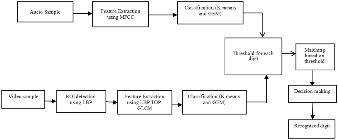
Block Diagram of proposed AV-ASR model using clustering method
Visual Speech Feature Extraction
LBP-TOP and GLCM: LBP is efficiently used in facial features extraction by dividing the face into a small region and extracting features from each region (Ahonen et al., 2006). It works as a local spatiotemporal descriptor to represent the isolated visual phrases of speech (Jain & Rathna, 2017). Texture description of every single region represents the appearance of that region (Ahonen et al., 2006). By combining all the region descriptors LBP method describes the global geometry of the image. Ojala et al. (2002) have introduced a grayscale and rotation invariant operator method in LBP. Besides all this research, nowadays it is efficiently used in visual speech recognition. Here, LBP technique is used to find out the ROI of the face. The example of LBP calculation is depicted in Fig. 2.
$$\begin{aligned} LBP_{(R,P)}= \sum _{p=0}^{p-1} t(n_p-n_c).2^p \end{aligned}$$
(1)
where \(n_p\) is the neighborhood pixels in each block, \(n_c\) is center pixels value. \(n_p\) is thresholded by its center pixels value \(n_c\). P is sampling points for 4 × 4 block P = 16. R is the radius for 4X4 block R = 2
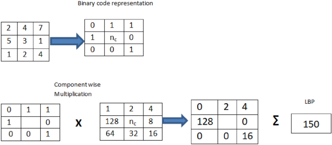
Example of LBP computation
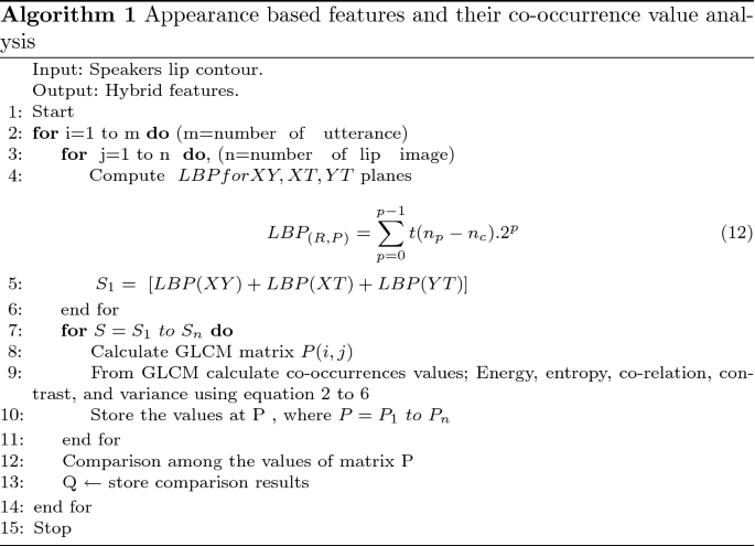
The whole face is divided into ten regions and after that features are extracted from every local region. It calculates the lip movement concerning time. One plane represents the appearance-based features in a spatial domain whereas the other two planes give the change of visual features with the time and features of motion in a time domain respectively. Histograms are generated from these three planes and add these three histograms to represent the appearance-based visual feature. GLCM is a gray level co-occurrence matrix used to extract second-order statistical texture features (Mohanaiah et al., 2013). Shikha et al. (2020) have used GLCM features to extract different image attributes like texture, color, and shape. In this paper, GLCM is used after LBP-TOP feature extraction. LBP-TOP matrix for each frame is used as an input for GLCM calculation. Energy, entropy, correlation, contrast, and variance are derived from the GLCM matrix. Therefore, five GLCM features are used here to differentiate different frames of particular utterance. Algorithm 1 represents the proposed feature extraction method.
Energy of GLCM is sum of the squared elements. The range of energy is [0 1]. For a constant picture, the energy is 1. The energy is calculated using equation 2.
$$\begin{aligned} Energy=~\underset{i,j=0}{\overset{I-1}{\mathop \sum }}\,P{{(i,j)}^{2}} \end{aligned}$$
(2)
where P(i,j) is the GLCM matrix, \(I=(0,1,2\ldots,I-1)\) are the distinct gray level intensities, calculate IXI order of GLCM, I is the number of gray levels in the image. Entropy is often used to represent visual texture and it is calculated using equation 3.
$$\begin{aligned} Entropy=~-\underset{i=0}{\overset{I-1}{\mathop \sum }}\,\underset{j=0}{\overset{I-1}{\mathop \sum }} \,P\left( i,j \right) \log ~(P\left( i,j \right) ) \end{aligned}$$
(3)
Correlation measures how correlated a pixel is to its neighbor for the entire image. Correlation is calculated from the equation 4.
$$\begin{aligned} Correlation=\frac{~\underset{i=0}{\overset{I-1}{\mathop \sum }}\,\underset{j=0}{\overset{I-1}{\mathop \sum }} \left( i,j \right) P\left( i,j \right) -{{\mu }_{~m~}}{{\mu }_{n}}}{{{\sigma }_{m}}{{\sigma }_{n}}} \end{aligned}$$
(4)
where \(\mu _m\), \(\mu _n\) and \(\sigma _m\), \(\sigma _n\) denote the mean and standard deviations of the row and column sums of the GLCM matrix P(i,j). Contrast and variance are calculated using equation 5 and 6 respectively. Over the entire image, contrast returns a measure of the intensity between a pixel and its neighbour.
$$\begin{aligned} Contrast= & {} ~\underset{i,j=0}{\overset{I-1}{\mathop \sum }}\,|i-j{{|}^{2}}P\left( i,j \right) \end{aligned}$$
(5)
$$\begin{aligned} Variance= & {} \underset{i,j=0}{\overset{I-1}{\mathop \sum }}\,{{\left( i-\mu \right) }^{2}}\log \left( P\left( i,j \right) \right) \end{aligned}$$
(6)
where \(\mu\) is the mean of the gray level distribution.
Audio Feature Extraction Using MFCC
The speech is rectified by the shape of the vocal tract, tongue, and teeth. This shape determines what type of sound will produce. The shape of the vocal tract is represented in the envelope of the short-time power spectrum and the job of MFCCs (Davis & Mermelstein, 1980; Soni et al., 2016) is to represent this envelope. Olivan et al. (2021) proposed a deep learning-based scheme along with mel-spectogram to detect music boundary. For calculating the MFCC, the following steps are followed:
- Step 1:
Analyse speech signal as a short frame.
- Step 2:
A window function is applied after framing.
- Step 3:
Discrete Fourier Transform (DFT) is used to convert the signal into the frequency domain.
- Step 4:
Apply Mel filter bank.
- Step 5:
The logarithm of Mel filter bank energies are taken.
- Step 6:
Convert Mel spectrum to the time domain.
The resultant coefficients are MFCCs. Here, 19 MFCCs are calculated as a speech feature vector.
Classification Using Clustering
Classification and dimension reduction is also an important task in this domain. Clustering is very useful for grouping and classifying data objects, especially for small data set. Therefore, K-means (Kanungo et al., 2002) and GEM (Nadif & Govaert, 2005) clustering techniques are used to cluster the audio-visual speech. First, K-means is used for the basic clustering and then GEM is used for the advanced clustering technique. GEM is also used because it is a soft clustering method and compares the results with K-means clustering. During training, the threshold is calculated for every digit and at the testing phase, measure the accuracy for each audio-visual digit. A boosting-aided adaptive cluster-based undersampling approach has been proposed by Devi et al. (2020) for class imbalance problem.
Revathi and Venkataramani (2009) have explored the effectiveness of perceptual features for recognizing isolated words and continuous speech. Lazli and Boukadoum (2017) have proposed an unsupervised iterative process for regulating a similarity measure to set the cluster's number and their boundaries. This has been developed for overcoming the shortcomings of conventional clustering algorithms, such as K-means and Fuzzy C-means which require prior knowledge of the number of clusters and a similarity measure.
K-means: K-means (Kanungo et al., 2002) is one of the simplest learning algorithms that solve the well-known clustering problem. It is a distance-based clustering algorithm. K-means creates the cluster in a circular shape because centroids are updated iteratively using the mean value. But if the data points distribution is not circular then the K-means algorithm becomes unsuccessful to generate the proper cluster.
GEM: GEM learning algorithm solves the uncertainty about the data points (Nadif & Govaert, 2005). GEM is a distribution-based clustering algorithm and overcomes the shortcomings of distance-based clustering. The working principle is based on the probability of data to determine the presence in a cluster. The Expectation-Maximization (EM) (Nadif & Govaert, 2005) algorithm is used in GEM to find the model parameter. The processes of GEM are discussed below:
- Step 1:
Initialize the mean \(\mu _k\), covariance \(\sigma _k\) and mixing coefficients \(\pi _k\) for cluster k, \(\mu _j\), covariance \(\sigma _j\) and mixing coefficients \(\pi _j\) for cluster j and evaluate the initial value of the log-likelihood.
- Step 2:
Expectation (E) step : Posterior probabilities of \(\gamma _j(x)\) is calculated using mean, covariance and mixture coefficients.
$$\begin{aligned} {{\text { }\!\!\gamma \!\!\text { }}_{\text {j}}}\left( \text {x} \right) =\frac{{{\text { }\!\!\pi \!\!\text { }}_{{{\text {k}}^{\!\!~\!\!\text { }}}}}.\text { }\!\!P\!\!\text { }\left( \text {x }\!\!|\!\!\text { }{{\text { }\!\!\mu \!\!\text { }}_{\text {k}}},{{\text { }\!\!\sigma \!\!\text { }}_{\text {k}}} \right) }{\mathop {\sum }_{\text {j}=1}{{\text { }\!\!\pi \!\!\text { }}_{\text {j}}}.\text { }\!\!P\!\!\text { }\left( \text {x }\!\!|\!\!\text { }{{\text { }\!\!\mu \!\!\text { }}_{\text {j},}}{{\text { }\!\!\sigma \!\!\text { }}_{\text {j}}} \right) } \end{aligned}$$
(7)
where x is the parameters collectively, \(\pi _k\) represent probability of belonging x to the k-th mixture component and \(\pi _j\) represent probability of belonging x to the j-th mixture component.
- Step 3:
Maximization (M) step:
$$\begin{aligned} {{\text { }\!\!\mu \!\!\text { }}_{\text {j}}}=\frac{\mathop {\sum }_{\text {n}=1}^{\text {N}}{{\text { }\!\!\gamma \!\!\text { }}_{\text {j}}}\left( {{\text {x}}_{\text {n}}} \right) {{\text {x}}_{\text {n}}}}{\mathop {\sum }_{\text {n}=1}^{\text {N}}{{\text { }\!\!\gamma \!\!\text { }}_{\text {j}}}\left( {{\text {x}}_{\text {n}}} \right) } \end{aligned}$$
(8)
where assign responsibility of a point \(x_n\) to exactly one cluster and N represents all the data.
$$\begin{aligned} {{\text { }\!\!\sigma \!\!\text { }}_{\text {j}}}=\frac{\mathop {\sum }_{\text {n}=1}^{\text {N}}{{\text { }\!\!\gamma \!\!\text { }}_{\text {j}}}\left( {{\text {x}}_{\text {n}}} \right) \left( {{\text {x}}_{\text {n}}}-{{\text { }\!\!\mu \!\!\text { }}_{\text {j}}} \right) {{({{\text {x}}_{\text {n}}}-{{\text { }\!\!\mu \!\!\text { }}_{\text {j}}})}^{\text {T}}}}{\mathop {\sum }_{\text {n}=1}^{\text {N}}{{\text { }\!\!\gamma \!\!\text { }}_{\text {j}}}\left( {{\text {x}}_{\text {n}}} \right) } \end{aligned}$$
(9)
$$\begin{aligned} {{\text { }\!\!\pi \!\!\text { }}_{\text {j}}}={{\text {N}}^{\text {T}}}\underset{\text {n}=1}{\overset{\text {N}}{\mathop \sum }}\,{{\text { }\!\!\gamma \!\!\text { }}_{\text {j}}}\left( {{\text {x}}_{\text {n}}} \right) \end{aligned}$$
(10)
- Step 4:
Estimate log likelihood.
- Step 5:
If not converged then return to step 2, i.e., Expectation and Maximization step.
$$\begin{aligned} \text {ln p}\left( \text {X }|\text { }\!\!\mu \!\!\text { },\text { }\!\!\sigma \!\!\text { },\text { }\!\!\pi \!\!\text { } \right) =\underset{\text {n}=1}{\overset{\text {N}}{\mathop \sum }}\,\text { ln }\!\!\text { }\left\{ \underset{\text {k}=1}{\overset{\text {k}}{\mathop \sum }}\,\underset{\text {k}}{\mathop \prod }\,\text { }\!\!P\!\!\text { }({{\text {x}}_{\text {n}}}|{{\text { }\!\!\mu \!\!\text { }}_{\text {k}}},{{\text { }\!\!\sigma \!\!\text { }}_{\text {k}}}) \right\} \end{aligned}$$
(11)
where \(\mu\), \(\sigma\), and \(\pi\) are the overall mean, covariance, and mixing coefficients respectively.
The E-step and the M-step are the two processes for the EM algorithm. The E-step is responsible for providing parameter values that compute the expected values of the latent variable. Based on the latent variable, M-step updates the parameters of the model.
Performance Analysis
Experimental Environment
Experiments are conducted in MATLAB, 2015 version. All the results and graphs are calculated in MATLAB. Different experiments are designed for a comprehensive assessment of the proposed system. The experiments are audio speech recognition using two different datasets and visual speech recognition using two different datasets.
For both the audio and visual speech recognition, results are obtained using two datasets and for each dataset, both the clustering and supervised machine learning algorithm are used. ANN, SVM, and NB are used separately to achieve the accuracy. All these experiments are conducted in different modules.
For audio speech recognition, 19 MFCC features are extracted and for visual speech recognition, LBP-TOP along with GLCM features are used. After feature extraction, the threshold value is calculated for the clustering algorithm in a training phase, which is described in "Performance Measure" section. In the testing phase, accuracy is measured with respect to the threshold value of each digit. Thus, the recognition rate is calculated for each individual digit for both audio and visual speech.
However, in a supervised machine learning algorithm, the recognition rate is calculated using correctly identified test sample and total supplied test sample which is described in "Results and Discussion" section.
The system is developed based on threshold value, if any one module will meet the threshold value then the system will accept the speech sample. Thus, disabled student can communicate with both the audio and visual speech and the system will provide the output using any one speech sample which is more convenient to the system.
Details of Dataset
Two datasets 'vVISWa' (Borde et al., 2004) and 'CUAVE' (Patterson et al., 2002) are used in this paper for experiments. Borde et al. (2004) have published a paper about the 'vVISWa' English digit dataset in 2016. The dataset is consisting of 0 to 10 English digits recorded in a laboratory. 'vVISWa' is consisting of 10 speakers including 6 males, and 4 females. Repetition of each digit is 10 times by individual speaker. 'CUAVE' is consisting of 0 to 10 English digits recorded from 18 male and 18 female speakers. A total of 1800 words have been recorded from the speaker. The database has been recorded in an isolated sound booth at a resolution of 720 \(\times\) 480 with the NTSC standard of 29.97 fps without any head movement.
Performance Measure
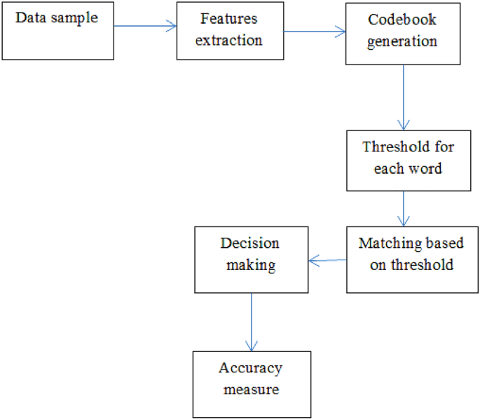
The threshold is generated for each digit using centroids obtained from the clustering algorithm. Codebook is generated for each repetition of a word and calculated the score by finding out the distance between codebook and feature vector. This score is considered as a parameter for testing the utterances. Euclidean distance is used to measure the score. The equation of calculating threshold is:
$$\begin{aligned} Threshold=\frac{{{\mu }_{1~}}{{\sigma }_{1~}}+{{\mu }_{2~}}{{\sigma }_{2}}}{{{\sigma }_{1}}+{{\sigma }_{2}}} \end{aligned}$$
(13)
where \(\mu _1\) is mean and \(\sigma _1\) is standard deviation of the tested sample. \(\mu _2\) is mean and \(\sigma _2\) is the standard deviation of the other randomly selected sample's codebook. This threshold is digit-specific. For robustness both claimed and random sample are considered to generate the threshold. The block diagrams of training and testing are depicted in Figs. 3 and 4, respectively.
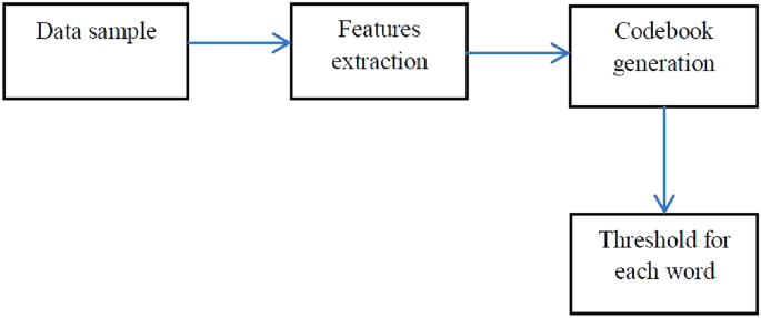
Block Diagram of training for AV-ASR using clustering
Block Diagram of testing for AV-ASR using clustering
Performance Measure for ANN, SVM, and NB is calculated using following method:
$$\begin{aligned} Recognition\,Rate= \frac{correctly~ identified~ test~ sample}{total~ supplied~ test~ sample} \times 100~\% \end{aligned}$$
(14)
Results and Discussion
Visual Speech Recognition Using Clustering Method
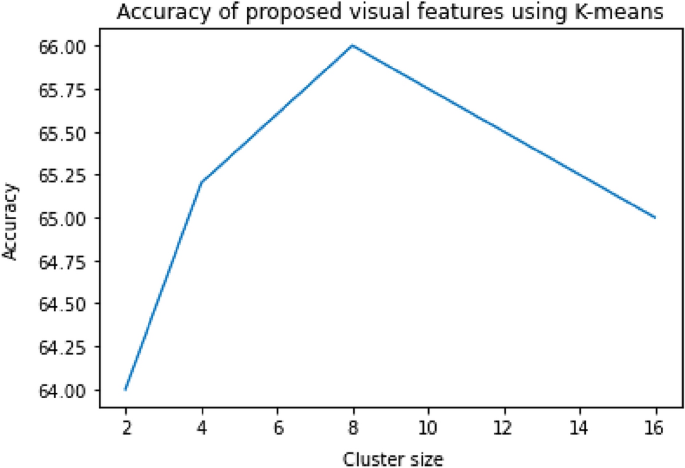
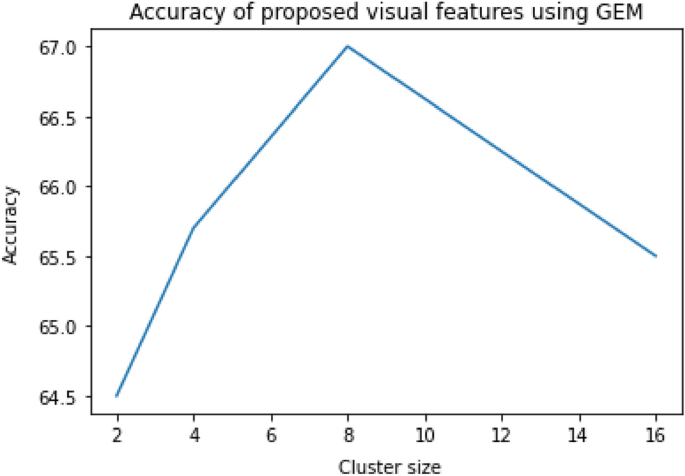
For the extraction of visual features, the primary move is to detect ROI, and here LBP is used for the detection of ROI. In this research, ROI is the speaker's lip contour and visual speech features are extracted from lip contour. Appearance-based features are extracted here along with second-order statistical analysis for visual speech recognition. The main motivation of the proposed feature extraction method is to capture dynamic visual information and co-occurrence values of features. Therefore, LBP-TOP along with GLCM features are proposed for visual speech recognition. LBP-TOP divides the ROI into sub-region and here, divides each ROI into 10 sub-regions, the dimension of each sub-region is 150. Therefore, the total dimension of the feature vector is (150X10), i.e., 1500 for each frame after extraction of LBP-TOP. LBP-TOP features are provided as input for GLCM calculation and energy, co-relation, contrast, variance as well as entropy statistical measures are extracted from these feature matrices. Here, energy gives the sum of the squared elements in the feature matrix, co-relation and contrast measure the co-relation and intensity contrast of a pixel to its neighbor. The calculated values can be −1 or 1 for positive or negative co-relation. The entropy is inversely proportional to GLCM energy and it achieves its largest value when all the elements of the given matrix are equal. After features extraction, K-means and GEM clustering algorithms are used for classification as well as dimension reduction. Cluster sizes 2, 4, 8, 16 are selected for both the K-means and GEM clustering algorithm. Accuracy increases with the increasing size of the cluster from 2 to 4 and 4 to 8. But accuracy drops down when cluster size increases from 8 to 16. This is because a higher cluster size shows the scattered representation of data which reduces the accuracy. The hard threshold is calculated for each speech sample. Tables 1 and 2 represent the proposed visual speech recognition using K-means and GEM. Here, the 'vVISWa' dataset is used.
Visual Speech Recognition Using ANN, SVM, and NB
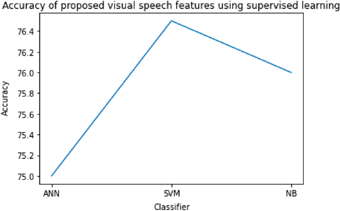
After features extraction, ANN (Kuncheva, 2004; Debnath & Roy, 2021), SVM (Debnath & Roy, 2021; Debnath et al., 2021), and NB (Debnath & Roy, 2021) machine learning algorithms are applied to recognize the visual speech. The visual speech is recognized using the different number of hidden nodes and two hidden layers in ANN. The system achieves 73.12 % recognition accuracy using 40, 30 number of hidden nodes. The experiments using SVM and NB are carried out with different kernel functions and the highest recognition accuracy of visual speech is obtained using the NB classifier, which is 74.23 %. The performance of visual speech recognition is calculated using 'vVISWa' dataset with different classifiers and shown in Tables 3 , 4, and 5, respectively. Figures 5, 6, and 7 represent the results obtained from the 'CUAVE' dataset.
Results of proposed visual speech features and K-means using 'CUAVE' dataset
Results of proposed visual speech features and GEM using 'CUAVE' dataset
Results of proposed visual speech features using 'CUAVE' dataset
Audio Speech Recognition Using Clustering
Here, 19 MFCC coefficients are extracted from audio speech. After feature extraction, classification using a clustering algorithm is performed for audio data.
Performance of audio speech recognition using K-means clustering is more than 90% for each digit. Accuracy increases with the increasing size of the cluster from 2 to 4 and drops down when cluster size increases from 4 to higher.
Using GEM the accuracy of audio speech recognition is more than 92% with k=4. Therefore, system performance depends on the cluster size for both the K-means and GEM clustering methods. Recognition accuracy for audio speech using clustering is represented in Tables 6 and 7.
Audio Speech Recognition Using ANN, SVM, and NB
The recognition of audio speech is also performed using ANN, SVM, as well as NB classifiers. For ANN, 2 hidden layers, 100 iterations, and the different number of hidden nodes are used for the experiment. SVM and NB machine learning approaches are applied based on the different kernel functions. The 'RBF'kernel function of SVM gives 93.55 % recognition accuracy whereas 92.19 % accuracy is obtained using the kernel function of NB. The accuracy is 91.32 % using 50, 40 hidden nodes with ANN. Tables 8, 9, and 10 are showing the performance of the proposed system using ANN, SVM, and NB. Figure 8 represents the accuracy obtained from 'CUAVE' dataset using both the clustering and supervised learning algorithm.
Integration of Audio-Visual Speech
Integration of two systems can be done using feature fusion and decision level fusion. Here, decision level fusion is considered for combining two systems. Individual word recognition rate is calculated for both audio and visual speech and then integrate two modalities for the better result. If one recognition model is failed, then the system considers the result from another model. Decision fusion provides better recognition rate for the overall system because each individual word is recognized as a token. For audio speech recognition, considered threshold rate is more than 85% and for visual speech recognition threshold is more than 70 %. Thus, when the accuracy is greater than or equal to the threshold, the input data is acceptable. Based on the threshold, when one of the recognition systems recognizes the respective input data of audio and visual speech, the system considers that speech gets recognized and provides the output.
Comparative Study
Visual speech features are extracted from the three orthogonal planes to capture the dynamic features. GLCM matrix is also calculated from LBP-TOP to measure second-order statistical features. The proposed features set consists of appearance-based visual features, the motion of lip, and the statistical measure of feature matrix which calculates the energy, contrast, correlation, variance, and entropy. K-means and GEM are used as an unsupervised and ANN, SVM, and NB are used as supervised machine learning methods. It is observed from the experiments that the proposed visual features provide a better recognition rate than the classical feature extraction method using both supervised and unsupervised methods. The comparison of results with the existing feature extraction method is shown in Table 11 using 'vVISWa' dataset and in Fig. 9, using 'CUAVE' dataset. The proposed method performs well because it calculates the statistical values from appearance features and gives more distinct information for visual speech. LBP has been used by many researchers for visual speech recognition but it does not capture the dynamic features of lip movement, for that reason researchers have proposed LBP-TOP to calculate features in a three-dimension. However, the co-occurrence values are also important, statistical value from the co-occurrence matrix gives distinguished feature.
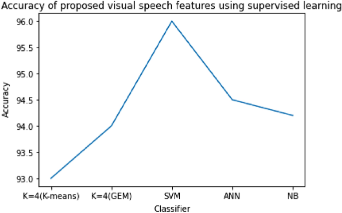
Results of audio speech rceognition using 'CUAVE' dataset
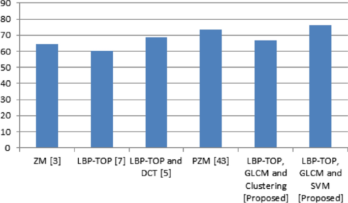
Comparison of proposed visual speech features with existing features using 'CUAVE' dataset
Conclusions and Future Work
The main focus of this paper is to provide AV-ASR based education system for physically challenged people. Because visual speech recognition is beneficial for ASR where background noise is more. To achieve this goal, LBP-TOP and GLCM are proposed for visual speech recognition. LBP-TOP captures the visual features in a spatio-temporal domain; therefore, the motion of the lip is also captured with appearance-based features. Five GLCM features are calculated to distinguish different frames of a particular utterance which is explained in the proposed methodology. After feature extraction, the classification of speech is also a challenging problem. It is observed that the proposed feature extraction method gives a better recognition rate for visual speech using a clustering algorithm and supervised machine learning algorithm. GEM is more efficient than K-means because it calculates gaussian distribution for clustering while K-means calculates the distance for generating clusters. Moreover, K-means fails to generate the right cluster when the distribution of data samples is not circular. Thus, the distribution-based model gives better performance instead of the distance measure model. Using supervised machine learning, SVM and NB give more accuracy than ANN visual speech recognition. In human-to-human communication, speech is a very natural and basic method. The design process for a speech user interface for human-computer interaction is presented in this paper using audio-visual data. In a noisy environment when the audio signal will not work the disabled people can communicate with the system using a visual speech signal. Further work can be designed for a hybrid visual feature extraction method to extract more robust features to develop for developing an AV-ASR-based education system.
References
-
Ahonen, T., et al. (2006). Face description with local binary patterns: Applications to face recognition. IEEE Transactions on Pattern Analysis and Machine Intelligence, 28(12), 2037–2041. https://doi.org/10.1109/TPAMI.2006.244.
-
Azeta, A., et al. (2010). Intelligent voice-based e-education system: A framework and evaluation. International Journal of Computing, 9, 327–334. https://doi.org/10.47839/ijc.9.4.726.
-
Borde, P., et al. (2004). 'vVISWa': A multilingual multi-pose audio visual database for robust human computer interaction. International Journal of Computer Applications, 137(4), 25–31. https://doi.org/10.5120/ijca2016908696.
-
Borde, P., et al. (2014). Recognition of isolated words using Zernike and MFCC features for audio visual speech recognition. International Journal of Speech Technology, 18(1), 23. https://doi.org/10.1007/s10772-014-9257-1.
-
Chen, R., et al. (2022). Image-denoising algorithm based on improved K-singular value decomposition and atom optimization. CAAI Transactions on Intelligence Technology, 7(1), 117–127. https://doi.org/10.1049/cit2.12044.
-
Dave, N. (2015). A lip localization based visual feature extraction method. Electrical & Computer Engineering, 4(4), 452. https://doi.org/10.14810/ecij.2015.4403.
-
Davis, S., & Mermelstein, P. (1980). Comparison of parametric representation for monosyllabic word recognition in continuously spoken sentences. IEEE Transactions on Acoustics, Speech, and Signal Processing, 28(4), 357–365. https://doi.org/10.1109/TASSP.1980.1163420.
-
Debnath, S., et al. (2021). Study of different feature extraction method for visual speech recognition. International Conference on Computer Communication and Informatics (ICCCI), 2021, 1–5. https://doi.org/10.1109/ICCCI50826.2021.9402357.
-
Debnath, S., & Roy, P. (2018). Study of speech enabled healthcare technology. International Journal of Medical Engineering and Informatics, 11(1), 71–85. https://doi.org/10.1504/IJMEI.2019.096893.
-
Debnath, S., & Roy, P. (2021). Appearance and shape-based hybrid visual feature extraction: Toward audio-visual automatic speech recognition. Signal, Image and Video Processing, 15, 25–32. https://doi.org/10.1007/s11760-020-01717-0.
-
Debnath, S., & Roy, P. (2021). Audio-visual automatic speech recognition using PZM, MFCC and statistical analysis. International Journal of Interactive Multimedia and Artificial Intelligence, 7(2), 121–133. https://doi.org/10.9781/ijimai.2021.09.001.
-
Devi, D., et al. (2020). A boosting-aided adaptive cluster-based undersampling approach for treatment of class imbalance problem. International Journal of Data Warehousing and Mining (IJDWM), 16(3), 60–86. https://doi.org/10.4018/IJDWM.2020070104.
-
Dupont, S., & Luettin, J. (2000). Audio-visual speech modeling for continuous speech recognition. IEEE Transaction on Multimedia, 2(3), 141–151. https://doi.org/10.1109/6046.865479.
-
Erber, N. P. (1975). Auditory-visual perception of speech. Journal of Speech and Hearing Disorders, 40(4), 481–492. https://doi.org/10.1044/jshd.4004.481.
-
Feng, W., et al. (2017). Audio visual speech recognition with multimodal recurrent neural networks. In International Joint Conference on Neural Networks (IJCNN), IEEE, pp. 681–688, 14-19. https://doi.org/10.1109/IJCNN.2017.7965918
-
Galatas, G., et al. (2012). Audio-visual speech recognition using depth information from the Kinect in noisy video conditions. In Proceedings of International Conference on Pervasive Technologies Related to Assistive Environments, ACM, pp. 1–4 https://doi.org/10.1145/2413097.2413100
-
Gao, J., et al. (2021). Decentralized federated learning framework for the neighborhood: A case study on residential building load forecasting. In Proceedings of the 19th ACM Conference on Embedded Networked Sensor Systems, ACM pp. 453–459. https://doi.org/10.1145/3485730.3493450
-
Ivanko, D., et al. (2021). An experimental analysis of different approaches to audio-visual speech recognition and lip-reading. In Proceedings of 15th International Conference on Electromechanics and Robotics, Springer, Singapore, pp. 197–209. https://doi.org/10.1007/978-981-15-5580-016
-
Jafarbigloo, S. K., & Danyali, H. (2021). Nuclear atypia grading in breast cancer histopathological images based on CNN feature extraction and LSTM classification. CAAI Transactions on Intelligence Technology, 6(4), 426–439. https://doi.org/10.1049/cit2.12061.
-
Jain, A., & Rathna, G. N. (2017). Visual speech recognition for isolated digits using discrete cosine transform and local binary pattern features. In IEEE Global Conference on Signal and Information Processing, IEEE, Montreal, pp. 368–372. https://doi.org/10.1109/GlobalSIP.2017.8308666
-
Jiang, R., et al. (2020). Object tracking on event cameras with offline-online learning. CAAI Transactions on Intelligence Technology, 5(3), 165–171. https://doi.org/10.1049/trit.2019.0107.
-
Kanungo, T., et al. (2002). An efficient k-means clustering algorithm: Analysis and implementation. IEEE Transactions on Pattern Analysis and Machine Intelligence, 24(7), 2037–2041. https://doi.org/10.1109/TPAMI.2002.1017616.
-
Kashevnik, A., et al. (2021). Multimodal corpus design for audio-visual speech recognition in vehicle cabin. IEEE Access, 9, 34986–35003. https://doi.org/10.1109/ACCESS.2021.3062752.
-
Kumar, L. A., et al. (2022). Deep learning based assistive technology on audio visual speech recognition for hearing impairedD. International Journal of Cognitive Computing in Engineering, 3, 24–30. https://doi.org/10.1016/j.ijcce.2022.01.003.
-
Kuncheva, I. (2004). Combining pattern classifiers: Methods and algorithms. Wiley.
-
Lazli, L., & Boukadoum, M. (2017). HMM/MLP speech recognition system using a novel data clustering approach. In IEEE 30th Canadian Conference on Electrical and Computer Engineering (CCECE), IEEE, Windsor. https://doi.org/10.1109/CCECE.2017.7946644
-
Mohanaiah, P., et al. (2013). Image texture feature extraction using GLCM approach. International Journal of Scientific and Research Publications, 3(5), 85.
-
Nadif, M., & Govaert, G. (2005). Block Clustering via the Block GEM and two-way EM algorithms. The 3rd ACS/IEEE International Conference on Computer Systems and Applications, IEEE. https://doi.org/10.1109/AICCSA.2005.1387029
-
Namasudra, S., & Roy, P. (2015). Size based access control model in cloud computing. In Proceeding of the International Conference on Electrical, Electronics, Signals, Communication and Optimization, IEEE, Visakhapatnam, pp. 1–4. https://doi.org/10.1109/EESCO.2015.7253753
-
Namasudra, S. (2020). Fast and secure data accessing by using DNA computing for the cloud environment. IEEE Transactions on Services Computing. https://doi.org/10.1109/TSC.2020.3046471.
-
Namasudra, S., & Roy, P. (2017). A new table based protocol for data accessing in cloud computing. Journal of Information Science and Engineering, 33(3), 585–609. https://doi.org/10.6688/JISE.2017.33.3.1.
-
Noda, K., et al. (2014). Audio-visual speech recognition using deep learning. Applied Intelligence, 42(4), 567. https://doi.org/10.1007/s10489-014-0629-7.
-
Ojala, T., et al. (2002). Multi resolution gray-scale and rotation invariant texture classification with local binary patterns. IEEE Transaction on Pattern Analysis and Machine Intelligence, 24(7), 971–987. https://doi.org/10.1109/TPAMI.2002.1017623.
-
Olivan, C. H., et al. (2021). Music boundary detection using convolutional neural networks: A comparative analysis of combined input features. International Journal of Interactive Multimedia and Artificial Intelligence, 7(2), 78–88. https://doi.org/10.48550/arXiv.2008.07527.
-
Patterson, E., et al. (2002). CUAVE: A new audio-visual database for multimodal human-computer interface research. In IEEE International Conference on Acoustics, Speech, and Signal Processing, IEEE, Orlando. https://doi.org/10.1109/ICASSP.2002.5745028
-
Rauf, H. T., et al. (2021). Enhanced bat algorithm for COVID-19 short-term forecasting using optimized LSTM. Soft Computing, 25(20), 12989–12999. https://doi.org/10.1007/s00500-021-06075-8.
-
Revathi, A., & Venkataramani, Y. (2009). Perceptual features based isolated digit and continuous speech recognition using iterative clustering approach networks and communication. In First International Conference on Networks & Communications, NetCoM., IEEE, Chennai. https://doi.org/10.1109/NetCoM.2009.32
-
Revathi, A., et al. (2019). Person authentication using speech as a biometric against play back attacks. Multimedia Tools Application, 78(2), 1569–1582. https://doi.org/10.1007/s11042-018-6258-0.
-
Shikha, B., et al. (2020). An extreme learning machine-relevance feedback framework for enhancing the accuracy of a hybrid image retrieval system. International Journal of Interactive Multimedia and Artificial Intelligence, 6(2), 15–27. https://doi.org/10.9781/ijimai.2020.01.002.
-
Shrawankar, U., & Thakare, V. (2010). Speech user interface for computer based education system. In International Conference on Signal and Image Processing, pp. 148–152. https://doi.org/10.1109/ICSIP.2010.5697459
-
Soni, B., et al. (2016). Text-dependent speaker verification using classical LBG, adaptive LBG and FCM vector quantization. International Journal of Speech Technology, 19(3), 525–536. https://doi.org/10.1007/s10772-016-9346-4.
-
Sui, C., et al. (2017). A cascade gray-stereo visual feature extraction method for visual and audio-visual speech recognition. Speech Communication, 90(1), 89. https://doi.org/10.1016/j.specom.2017.01.005.
-
Zhao, G., et al. (2009). Lipreading with local spatiotemporal descriptors. IEEE Transactions on Multimedia, 11(7), 56. https://doi.org/10.1109/TMM.2009.2030637.
Source: https://link.springer.com/article/10.1007/s10803-022-05654-4
0 Response to "Audio visual Speech Modeling for Continuous Speech Recognition"
Post a Comment